[General purpose grid generation tool]
Create grids by solving convergence calculation.
Grids generated by this alogrithm consists of cells whose edge lengths changes smoothly, so it helps solvers do stable simulations.
An advantage of this tool is that there is no limitation about the number of division lines in streamwise and cross section directions. Because of this feature, user can use this algorithm to define grids with low-water channels, or for junctions of rivers.
Figure 305 to Figure 308 shows examples of grids generated with the algorithm.
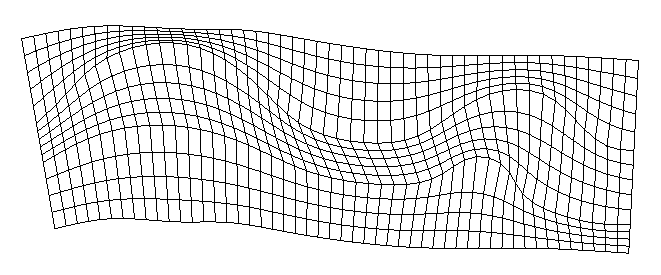
Figure 305 Example of a grid created by general purpose grid generation tool (1)
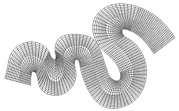
Figure 306 Example of a grid created by general purpose grid generation tool (2)

Figure 307 Example of a grid created by general purpose grid generation tool (3)
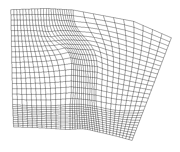
Figure 308 Example of a grid created by general purpose grid generation tool (4)
When this algorithm is selected, if a river survey data is imported, The dialog in Figure 309 is shown.
When you specify the number of Control Cross Sections and click on [OK] button, center line is defined by using the river center lines of river survey data, as shown in Figure 310.
If a river survey data is not imported, user can define the center line with mouse operations.
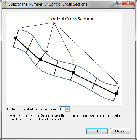
Figure 309 [Specify the Number of Control Cross Sections] dialog
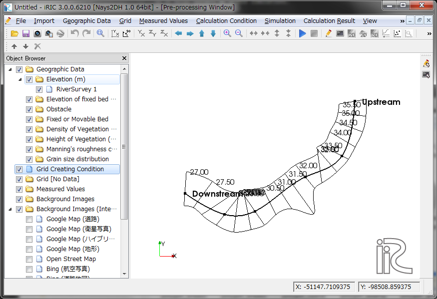
Figure 310 Example of center line
Next, please generate left bank line and right bank line. Select [Build Left bank and Right bank lines] from menu. [Build Bank Lines] dialog (Figure 311) will be shown. When you input the distance on the dialog and click on [OK], Left bank line and Right bank line are generated, and shown like in Figure 312.

Figure 311 [Build Bank Lines] dialog
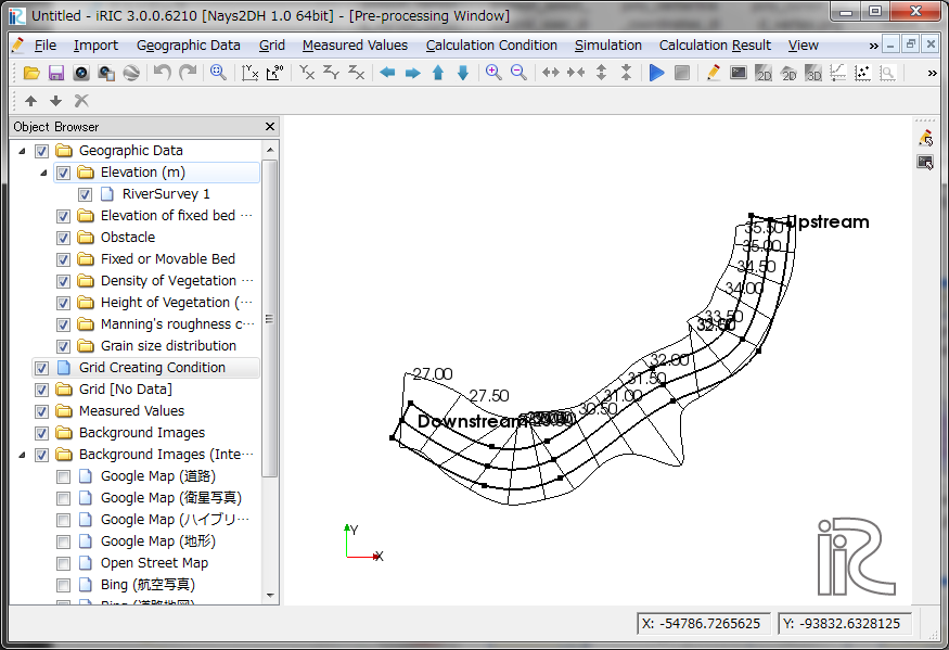
Figure 312 Example of generated Left bank line and Right bank line
After you defined left bank and right bank lines, you can edit the points, or divide the region, if you need to.
When you’ve finished defining the region to generate grid, select the following:
Menu: [Grid] (G) –> [Create Grid] (C)
[Division Setting for Whole Region] dialog (Figure 313) will be shown, so imput the numbers of divisions for streamwise direction and cross section direction, and click on [OK] button, to generate grid like Figure 314.
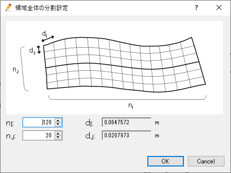
Figure 313 [Grid generation] dialog
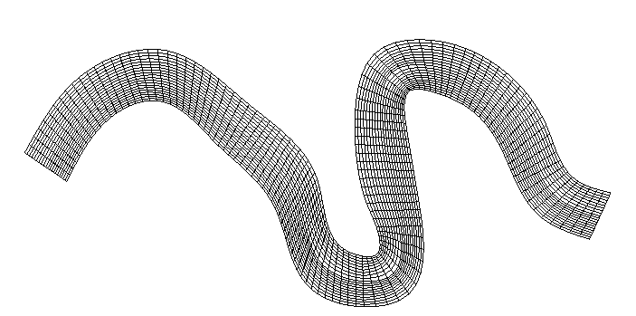
Figure 314 Example of generated grid
In cases you wan to generate simple grids, the workflow is simple as above, but general purpose grid generating tool allow you to control the cell edge lengths and grid node positions more precisely. Please refer to the following sections to know how to do that.
[Build Left bank and Right bank lines] (B)
Description: Generate Left bank and Right bank lines.
Dialog in Figure 311 is shown, so specify the distance values and click on [OK].
Figure 312 shows an example of generated [Left Bank Line] and [Right Bank Line].
You can modify the lines by dragging the vertices.
[Add Vertex] (A)
Description: Add vertices to lines
When you move the mouse cursor to hover on lines after selecting this menu, the mouse cursor changes to the shape in Figure 315.
Left click on the line and drag it to add a new vertex. The vertex is placed wherever you release the left click button.

Figure 315 The mouse cursor display when adding a vertex is possible
[Remove Vertex] (R)
Description: Deletes the vertex of lines.
When this is selected and you move the cursor onto the vertex of the lines, the cursor shape will change (Figure 316). Left clicking will remove the vertex.

Figure 316 The mouse cursor when removing the vertex is possible
[Edit Coordinates] (E)
Description: Edits the coordinates of the line currently selected.
When you select the menu, the [Line Coordinates] dialog (Figure 317) will open. Edit the coordinates and click on [OK].
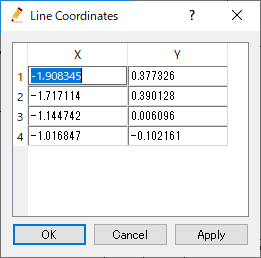
Figure 317 [Line Coordinates] dialog
[Create Grid] (C)
Description: Crreate grid by inputting division setting.
[Division Setting for Whole Region] dialog (Figure 313) is shown, so input the number of divisions, and click on [OK] button. In [dI] and [dJ], the average cell width in I-direction and J-direction are displayed.
When you’ve specified division settings for lines, using [Division Setting for selected line], the dialog is not shown, and grid is generated based on the settings.
When you select [Clear division Setting], division settings on all lines are removed, and the dialog will be shown again, when selecting the menu.
[Add Division line] (D)
Description: Add a division line inside the region.
When in the mode to add division line, when user moves the mouse cursor to the outer edge line of the region, the mouse cursor changes to the shape in Figure 315. When user clicks the left mouse button, a new point is created on the line, and user can start defining new division line.
User can add points to define a poly line, and when user moved the mouse cursor to the edge on the other side, the mouse cursor changes to the shape in Figure 315 again. When user click the left mouse button, the definition of the new line is finished, and the region is devided.
You can divide the region with arbitrary number of lines, both in streamwise direction and cross section direction.
An example of before and after dividing a region is shown in Figure 318 and Figure 319.
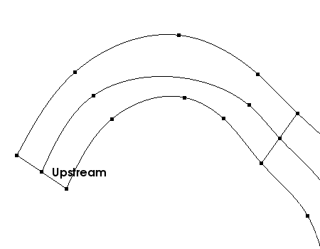
Figure 318 Example of display before adding division line
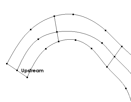
Figure 319 Example of display after adding division line
[Remove Division line] (I)
Description: Remove the division line currently selected, to join the two regions separated by that line.
To select this menu, user have to select a division line inside the region first.
When user selec the menu, [Warning] dialog (Figure 320) is shown. When user click on [Yes] button, removing the division line is executed.
An example of before and after removing division line is shown in Figure 321 and Figure 322.
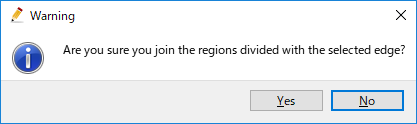
Figure 320 [Warning] dialog
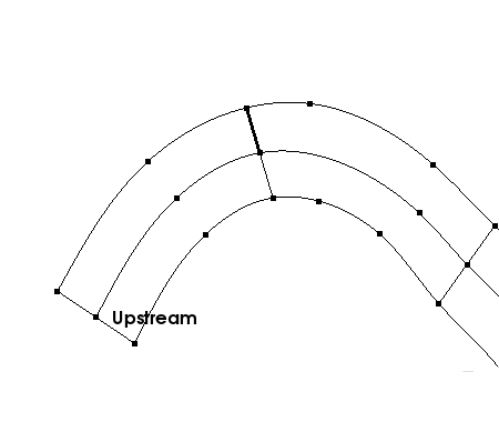
Figure 321 Example of display before removing a division line
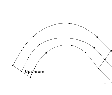
Figure 322 Example of display after removing a division line
[Division Setting for selected line] (D)
Description: Edit the division setting for the line currently selected.
Please select the line on which you want to edit division setting, by clicking it. The selected line is shown as a bold line.
[Division Setting] dialog (Figure 323) is shown, so edit the setting and click on [OK] button.
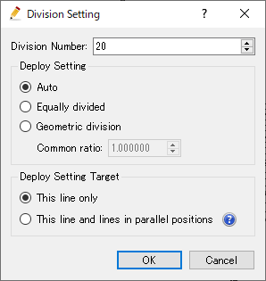
Figure 323 [Division Setting] dialog
Note
About [Auto] setting in [Deploy Setting]
When you select [Auto] in [Deploy Setting], the division points are deployed on the line like below:
The points are deployed on the line with [Geometric division] setting.
The [Common ratio] value is calculated by solving convergence calculation, to make the ratio between the cell widths at the region boundaries near to 1.
Using [Auto] setting, you can generate grids in which the grid cell widths changes smoothly on grid edges. But in cases you’ve specified extreme settings as division numbers, the [Common ratio] values are calculated to be big value. In such cases the grid generated are not appropriate for calculation.
In such cases, please specify the [Deploy Setting] manually, by selecting [Equally divided] or [Geometric division].
Note
About [Deploy Setting Target]
[Deploy Setting Target] is [This line only] in default, but you can select [This line and lines in parallel positions].
When you select [This line and lines in parallel positions], for example when you’ve selected a line with streamwise direction, the same setting is applied to the lines that exists on the left bank side and right bank side.
[Deploying Setting for selected area] (D)
Description: Edit the points deploying setting for the area currently selected.
Before selecting the menu, select the area you want to edit deploying setting, by clicking on the region. The selected area is painted gray.
[Points Deploying Setting] dialog (Figure 324) is shown, so edit the points deploying setting, and click on [OK] button.
As shown on the dialog, the points deploying setting cah be selected from the followings:
[Ratio]
[Poisson]
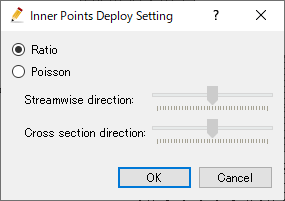
Figure 324 [Points Deploying Setting] dialog
Note
About [Deploying Setting]
For each setting, the points are deployed with the algorithms below:
[Ratio]: The point positions are calculated by solving convergence calculation, so that the grid cell edge lengths changes smoothly.
[Poisson]: The point positions are calculated by solving poisson equation. By moving the sliders with labels [Streamwise direction] and [Cross section direction], you can control the position of points precisely, to move the points to left bank side or right bank side, for example.
[Clear Division Setting] (C)
Description: Clear the division setting all lines.