iRIC functions
iRIC functions can be categorized into the seven groups below:
Editing geographic data
Creating grids
Editing grids
Loading measured data
Setting calculation conditions
Lunching a solver
Visualizing the calculation results
Making a graph
The abstract of each function groups are explained in the following sections.
Editing geographic data
Geographic data handles coordinates of data and the attributes at that coordinates, such as elevation, vegetation type, vegetation density, land use. You can import and edit geographic data with iRIC.
Geographic data are used to determine the attributes at each node or cell by interpolation. You can use cross-section data also for creating a grid.
The attributes that you need to input differ by the solver you use.
iRIC can import and edit four types of geographic data:
Point cloud data
Cross-section data
Raster data
Time series raster data
Polygons
Lines
Points
Figure 23, Figure 24, Figure 25, Figure 26, Figure 27 and Figure 28 show example of [Point Cloud Data], [Cross-Section Data], [Raster Data], [Polygons], [Lines] and [Points] respectively.
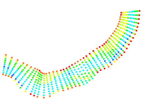
Figure 23 Example of [Point Cloud Data]
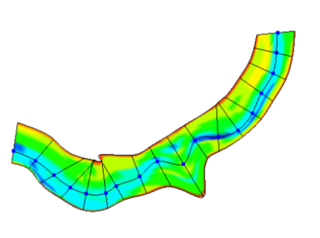
Figure 24 Example of [Cross-Section Data]
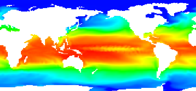
Figure 25 Example of [Raster Data]
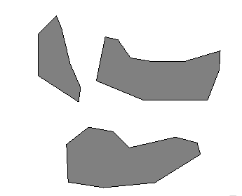
Figure 26 Example of [Polygons]
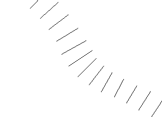
Figure 27 Example of [Lines]
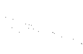
Figure 28 Example of [Points]
Refer to [Geographic Data] for detail.
Creating a grid
You can create the grid that the solver uses. A grid can be created in two steps:
Determine the grid shape (coordinates of each node).
Determine the node/cell attributes by interpolating geographic data.
In step 1., you select one of the algorithms that can produce the grid that the solver requires, and then, you create a grid by specifying grid creating condition.
Step 2. is automatically done. iRIC does this step automatically by recognizing the type of geographic data, and selecting the appropriate algorithm for interpolation for that type.
iRIC can create grids of the following types:
Two-dimensional structured grid
Two-dimensional unstructured grid
One-dimensional structured grid (Each node holds sectional data.)
Refer to Grid creating functions for details.
Editing the grid
You can edit the grid. You can do the following operations:
Editing the grid shape (the coordinates of each node)
Editing the attributes of each node or cell
Refer to Editing the grid for the details.
Loading measured data
You can load measured data from text files, to use it as background data for creating data, or to compare with calculation results. You can do the following operations:
Importing measured data from text files
Editing display settings of measured data
Refer to [Measured Data] (M) for the details.
Setting the calculation conditions
You can set the calculation conditions. The calculation conditions differ by the solver selected.
Refer to [Calculation Conditions] for the details.
Launching the solver
You can launch the solver and monitors the simulation status using [Solver Console]. You can stop calculations when you want to. Figure 29 shows an example of the [Solver Console] that displays solver outputs.
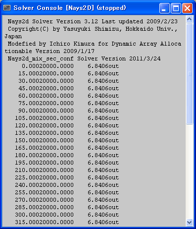
Figure 29 [Solver Console]
Refer to [Simulation] (S) for details.
Post-processing
You can visualize the calculation results that the solver output. You can use [2D Post-processing Window] (Figure 30), [Bird’s-Eye 2D Post-processing Window] (Figure 31), and [3D Post-processing Window] (Figure 32) for that purpose.
Refer to Visualization functions for details.
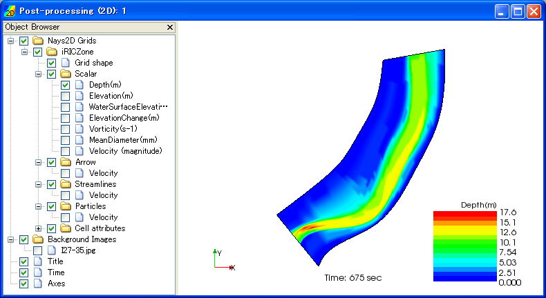
Figure 30 [2D Post-processing Window]
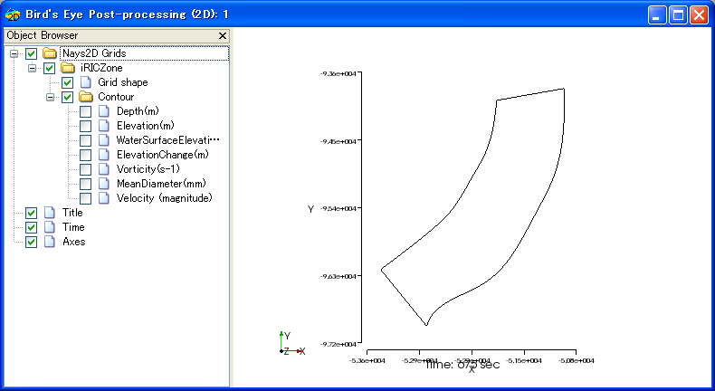
Figure 31 [Bird’s-Eye 2D Post-processing Window]
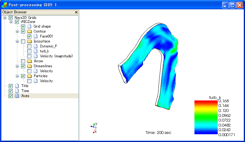
Figure 32 [3D Post-processing Window]
Making a graph
You can display graphs with the calculation results that the solver output, using [Graph Window] (Figure 33) and [Scattered Chart Window] (Figure 34).
Refer to Making a graph for details.
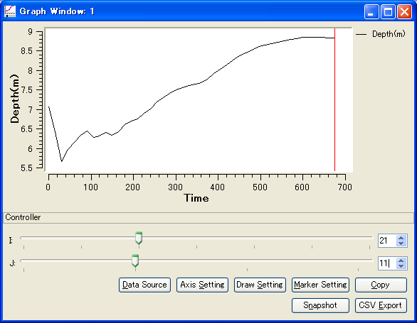
Figure 33 [Graph Window]
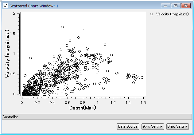
Figure 34 [Scattered Chart Window]