2D visualization functions
The functions for visualizing the 2D calculation results are explained.
Use [2D Post-processing Window] for 2D visualization of simulation results as explained below.
[Open New 2D Post-processing Window]
Either of the following actions opens a new [2D Post-processing Window].
Menu bar: [Calculation Results] (R) –> [Open New 2D Post-processing Window]
Operation Toolbar: ![]()
The new [2D Post-processing Window] (Figure 386) will open.
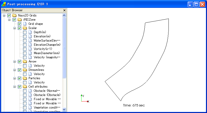
Figure 386 [2D Post-processing Window]
[Object Browser]
Figure 387 shows an example of the [Object Browser] of [2D Post-processing Window].
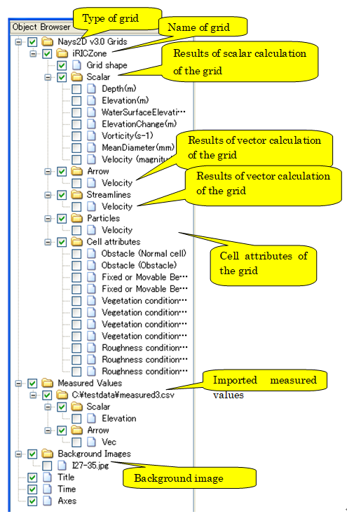
Figure 387 The [Object Browser] of the [2D Post-processing Window]
Settings on the elements shown in the [Object Browser] of [2D Post-processing Window] can be edited mainly from [Draw] menu and [Measured Data] menu. For operations on [Axes] and [Distance Measures], refer to [Axes] and [Distance Measures] respectively.
Note
In iRIC 4.1 and later, the input grid can be displayed in the [2D Post-processing Window]. The input grid display settings are the same as in the preprocessor. See Display Settings for more details.
[Attribute Browser]
You can use [Attribute Browser] to see the values of attributes defined at grid nodes.
Figure 388 shows an example of [Attribute Browser].
You can open [Attribute Browser] with the following operations:
Menu bar: [View] (V) -> [Attribute Browser] (A)
Right-clicking menu: Select [Scalar (node)] etc. in [Object Browser], and select [Show Attribute Browser] from right-clicking menu.
While [Attribute Browser] is shown, you can do the following operations using mouse:
When no point is selected, you can see the values of attributes defined at the grid node, by moving the mouse cursor. The attribute values defined at the point nearest to the mouse cursor is shown continuously. The grid node which is selected to show attributes is highlighted with a big black square.
If you left-click on grid node when values are shown in [Attribute Browser], the grid node is selected, and values at that point is shown, until you select another point or clear selection. When you left-click on another grid node, the new node is selected.
If you left-click on point which is outside or the region where calculation result is defined, selection is cleared.
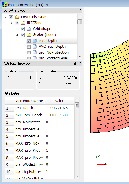
Figure 388 Example of [Attribute Browser]
[Grid Shape] (G)
Description: Sets the grid shape settings.
When you select [Grid Shape], the [Grid Shape Setting] dialog (Figure 389) will open. Set it and click on [OK]. Figure 390 shows examples of the display when the setting is for [Wireframe] and [Grid line], respectively.
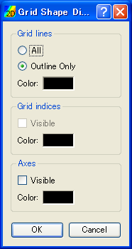
Figure 389 [Grid Shape] dialog

Figure 390 Examples of graphics displayed by the [Grid Shape] setting
[Contour (nodes)] (C)
Description: Sets the contour settings for calculation results defined at grid nodes.
When you select [Contour], the [Contour Setting] dialog (Figure 391) will open. Set it and click on [OK].
When you click on [Region Setting] button, [Region Setting] dialog (Figure 392 or Figure 393) will open.
When you click on [Color Bar Setting] button, [Color Legend Setting] dialog (Figure 394) will open.
Please refer to [Color Setting] about the dialog that is shown when you select [Custom] as [Colormap] and click on [Setting] button.
Figure 395 shows an example of displayed contours for each [Display Setting] setting.
With iRIC 3.0, it is now possible to visualize contours for multiple calculation results at the same time. To visualize multiple contours, please check on the check boxes for multiple items in the object browser.

Figure 391 [Contour Setting] dialog
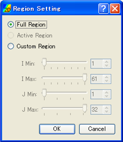
Figure 392 [Region Setting] dialog (Structured grid)
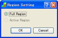
Figure 393 [Region Setting] dialog (Unstructured grid)
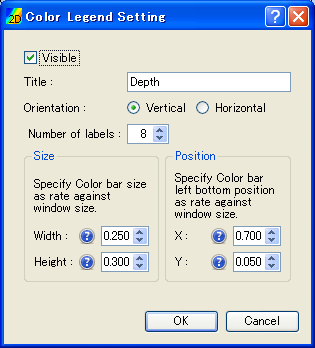
Figure 394 [Color Legend Setting] dialog
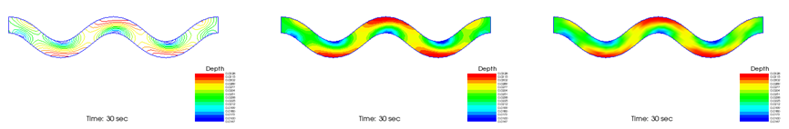
Figure 395 Examples of the contour display by the [Display Setting] setting
[Contour (Cell center)] (L)
Description: Sets the contour settings for calculation Results defined at cell centers.
When you select [Contour], the [Contour Setting] dialog (Figure 396) will open. Set it and click on [OK].
When you click on [Region Setting] button, [Region Setting] dialog (Figure 397 or Figure 398) will open.
When you click on [Color Bar Setting] button, [Color Legend Setting] dialog (Figure 399) will open.
Please refer to [Color Setting] about the dialog that is shown when you select [Custom] as [Colormap] and click on [Setting] button.
Figure 400 shows an example of displayed contours for each [Display Setting] setting.
With iRIC 3.0, it is now possible to visualize contours for multiple calculation results at the same time. To visualize multiple contours, please check on the check boxes for multiple items in the object browser.
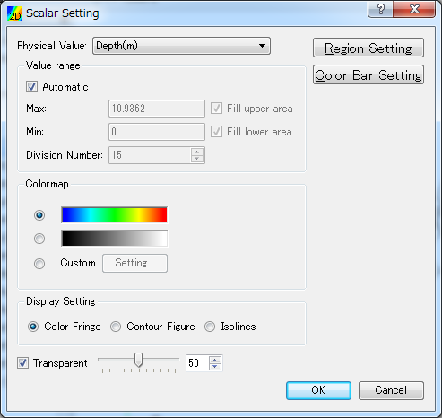
Figure 396 [Contour Setting] dialog
Figure 397 [Region Setting] dialog (Structured grid)
Figure 398 [Region Setting] dialog (Unstructured grid)
Figure 399 [Color Legend Setting] dialog
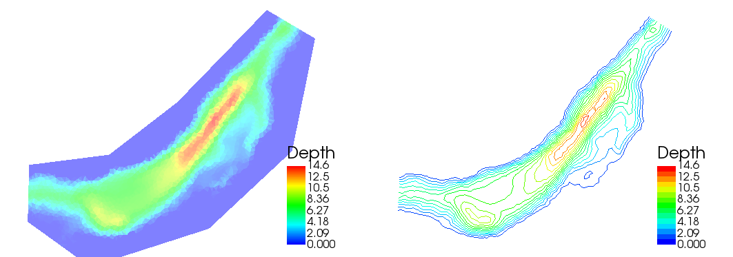
Figure 400 Examples of the contour display by the [Display Setting] setting
[Contour (edgeI)], [Contour (edgeJ)]
Description: Sets the contour settings for calculation Results defined at i-direction edges and j-direction edges.
From the values defined at grid edges, values at grid nodes are calculated by interpolation, and contour is drawn with values at grid nodes.
The function to edit setting of contours is the same to the contour function for grid nodes. Refer to [Contour (nodes)] (C) for detail.
[Arrow] (A)
Description: Sets the [Arrow] display.
When you select [Arrow], the [Arrow Setting] dialog (Figure 401 or Figure 402) will open. Set it and click on [OK]. Figure 405 shows an example of the [Arrow] display.
Figure 401 [Arrow Setting] dialog (structured)
Figure 402 [Arrow Setting] dialog (unstructured)
Figure 403 [Region Setting] dialog (Structured grid)
Figure 404 [Region Setting] dialog (Unstructured grid)
Figure 405 Example of the [Arrow] display
[Streamline] (S)
Description: Sets the streamline settings.
When you select [Streamline], the [Streamline Setting] dialog (Figure 406 or Figure 407) will open. Set it and click on [OK]. Figure 408 shows an example of the streamline display.
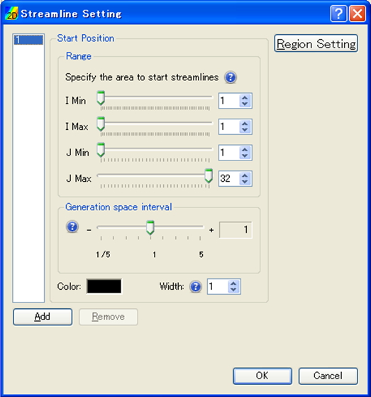
Figure 406 [Streamline Setting] dialog (Structured)
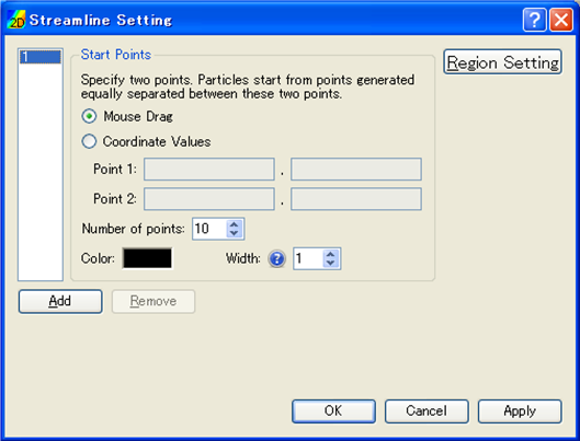
Figure 407 [Streamline Setting] dialog (Unstructured)
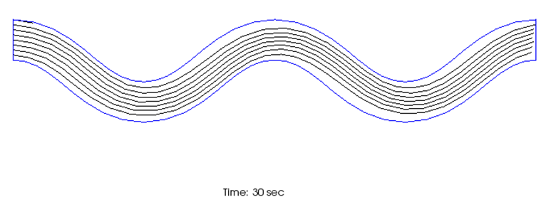
Figure 408 Example of the [Streamline] display
[Particles (auto)] (P)
Description: Sets the particle settings.
[Particles (auto)] is the function to generate particles in GUI, and simulate where where the particles will move to, using velocity in calculation result, and visualize the particles.
When you select [Particles], the [Particle Setting] dialog (Figure 409 or Figure 410) will open. Set it and click on [OK]. Figure 411 shows an example of the [Particles] display.
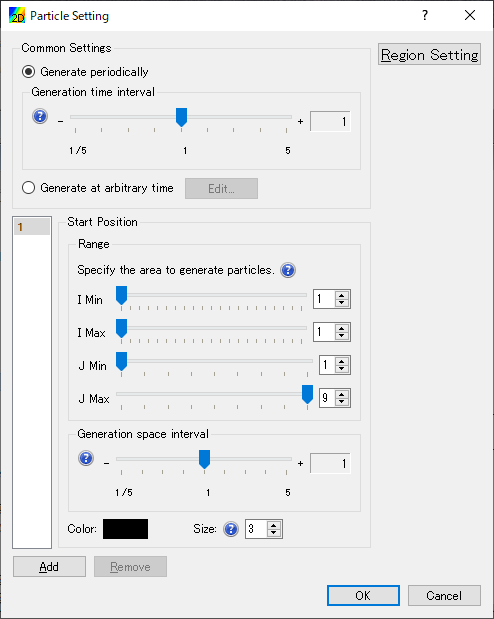
Figure 409 [Particle Setting] dialog (Structured)
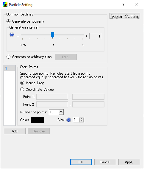
Figure 410 [Particle Setting] dialog (Unstructured)
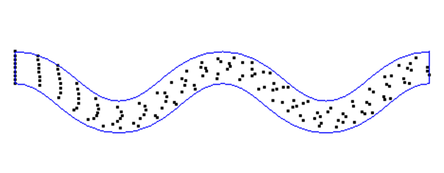
Figure 411 Example of the [Particles] display
[Particles] (R)
Description: Sets the particle settings.
[Particles] is the function to load particles output by solber, and visualize the particles.
When scalar attributes are output, user can change particle colors. When vector attributes are output, user can show arrows.
When you select [Property] menu in right-clicking menu of [Scalar] and [Vector] Folder under [Particles], the dialogs in Figure 412, Figure 413 will be shown. Please edit the setting, and click on [OK] button.
Figure 414 shows an example of the [Particles] display.
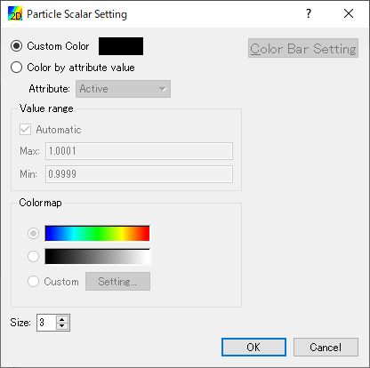
Figure 412 [Particle Scalar Setting] dialog
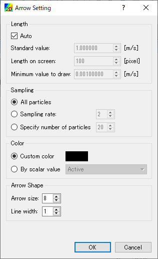
Figure 413 [Arrow Setting] dialog
Figure 414 Example of the [Particles] display
[Polygons] (O)
Description: Sets the polygon settings
You can open polygon settings dialog, when user select the folder under “Polygon” folder in the [Object Browser].
When you select [Polygons], the [Polygon Setting] dialog (Figure 415) will open. Update setting and click on [OK]. Figure 416 shows an example of the [Polygons] display.
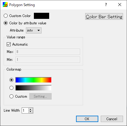
Figure 415 [Polygon Setting] dialog

Figure 416 Example of the [Polygons] display
[Cell Attributes] (C)
Description: Sets the cell color and the order of display for cell attributes.
When you select [Cell Attributes], the [Cell Attributes] dialog (Figure 417) will open. Set it and click on [OK].

Figure 417 [Cell Attributes] dialog
[Label]
Description: Show label based on calculation result values.
Label is the function to show label string defined using calculation results at grid nodes, cells, edges, etc.
Figure 418 shows an example of label.
Refer to Label display function for detail.
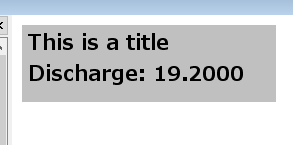
Figure 418 Example of [Label] display
[Background Image]
Description: Shows background images.
This function is same to the function implemented on Pre-processor Window. Please refer to Background Image for detail.
[Background Image (Internet)]
Description: Shows background images got from Internet.
This function is same to the function implemented on Pre-processor Window. Please refer to [Background Images (Internet)] for detail.
[Title] (T)
Description: Sets the title settings.
When you select [Title], the [Title Setting] dialog (Figure 419) will open. Set it and click on [OK].
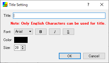
Figure 419 [Title Setting] dialog
[Time] (M)
Description: Sets the time settings.
When you select [Time], the [Time Setting] dialog (Figure 420) will open. Set it and click on [OK].
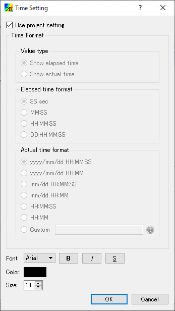
Figure 420 [Time Setting] dialog
[Measured Data] (M)
The functions related to [Measured Data] that are available in [2D Post-processing Window] are the same to those in [Pre-processing Window]. Refer to [Measured Data] (M).