3D visualization functions
Below are the functions for visualizing the 3D calculation results.
Use [3D Post-processing Window] for 3D visualization of simulation results as explained below.
[Open New 3D Post-processing Window]
Either of the following actions opens a new [3D Post-processing Window].
Menu bar: [Calculation Results] (R) –> [Open New 3D Post-processing Window]
Operation Toolbar: Select 
The new [3D Post-processing Window] (Figure 462) will open.
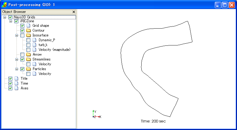
Figure 462 [3D Post-processing Window]
[Object Browser]
Figure 463 shows an example of the [Object Browser] of [3D Post-processing Window].
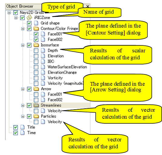
Figure 463 The [Object Browser] of the [3D Post-processing Window]
Settings on the elements shown in the [Object Browser] of [3D Post-processing Window] can be edited mainly from [Draw] menu. For operations on [Axes], refer to [Axes].
[Grid Shape] (G)
Description: Setup the grid shape settings.
When you select [Grid Shape], the [Grid Shape Setting] dialog (Figure 464) will open. Set it and click on [OK]. Figure 465 shows examples of the display when the setting is for [Wireframe] and [Grid line], respectively.
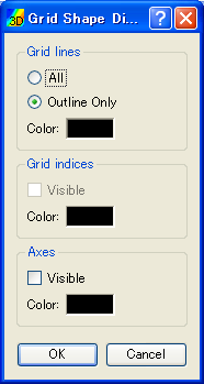
Figure 464 [Grid Shape] dialog
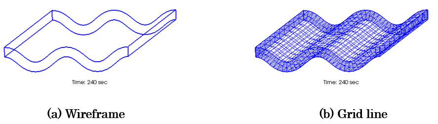
Figure 465 Examples of graphics displayed by the [Grid Shape] setting
[Contours] (C)
Description: Setup the contour settings.
When you select [Contour], the [Contour Group Setting] dialog (Figure 466) will open. Setup the setting, and click on [OK]. Figure 468 shows examples of the contour display for the [Counter] setting.
Please refer to [Color Setting] about the dialog that is shown when you select [Custom] as [Colormap] and click on [Setting…] button.
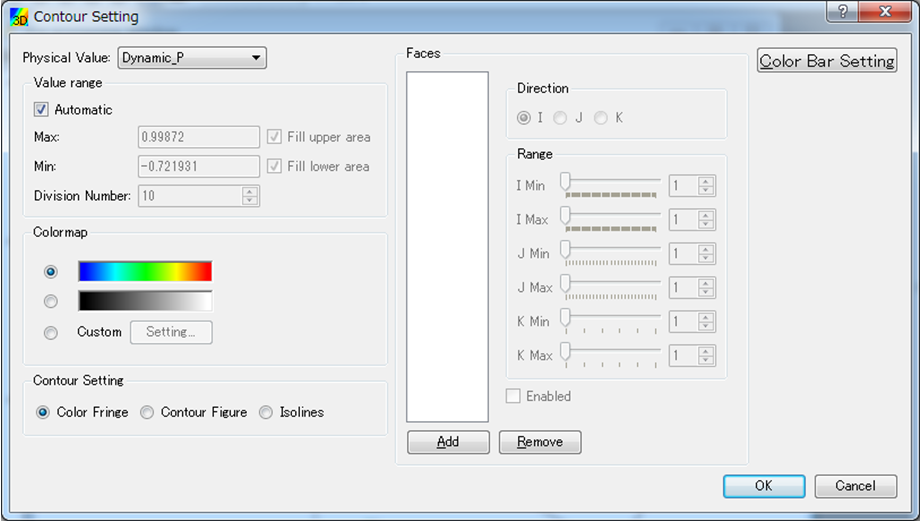
Figure 466 [Contour Group Setting] dialog
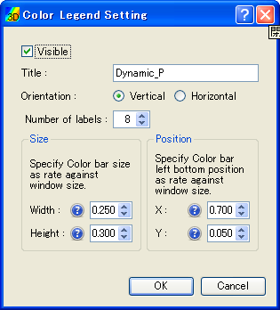
Figure 467 [Color Legend Setting] dialog

Figure 468 Examples of the contour display by the [Display Setting] setting
[Iso Surface]
Description: Setup the iso-surface settings.
When you select [Iso Surface], the [Iso Surface Setting] dialog (Figure 469) will open. Set it and click on [OK]. Figure 470 shows examples of the iso surface display.
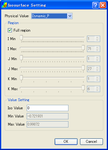
Figure 469 [Iso Surface Setting] dialog
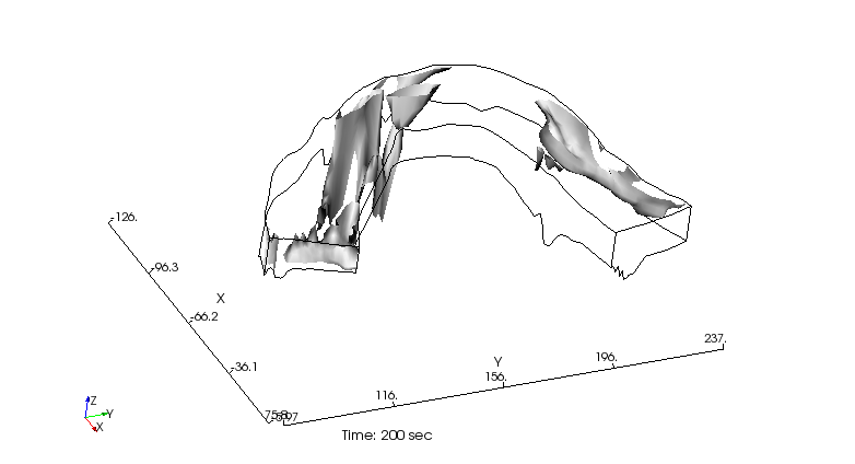
Figure 470 The Isosurface example
[Contours (cell center)]
Description: Setup the contour setting for values output at cell centers.
When you select [Contours (cell center)], the [Contour Setting (cell center)] dialog (Figure 471) will open. Setup the setting, and click on [OK].
Please refer to [Color Setting] about the dialog that is shown when you select [Custom] as [Colormap] and click on [Setting…] button.
Figure 472 shows an exampl.
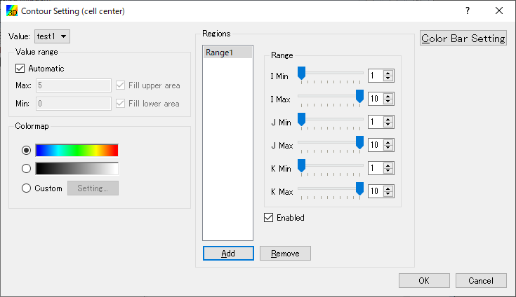
Figure 471 [Contour Setting (cell center)] dialog
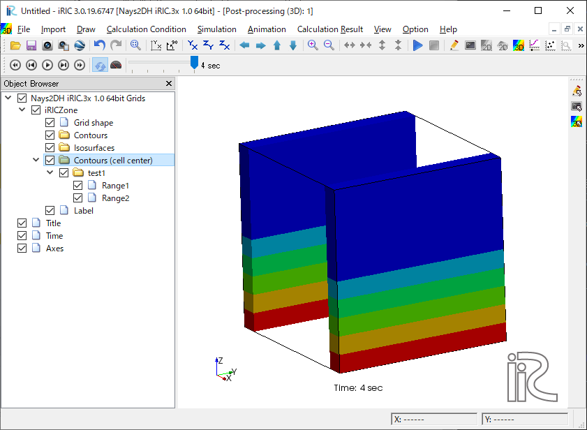
Figure 472 Example of [Contours (cell center)]
[Arrows] (A)
Description: Setup the arrow (or vector) group settings.
When you select [Arrow], the [Arrow Group Setting] dialog (Figure 473) will open. Set it and click on [OK]. Figure 474 shows an example of the [Arrow] display.
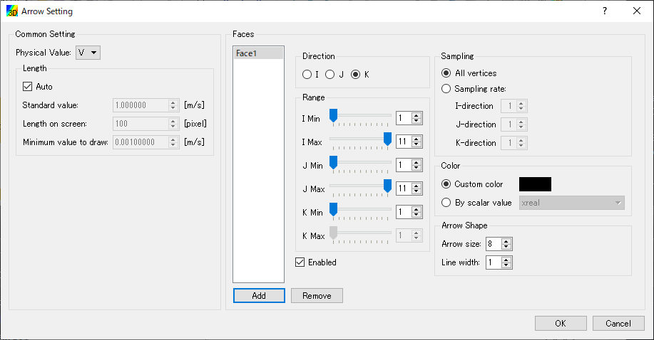
Figure 473 [Arrow Group Setting] dialog
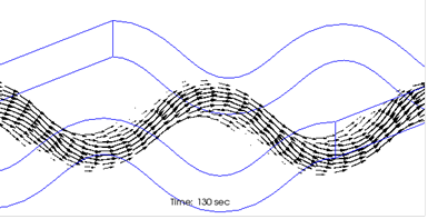
Figure 474 Example of the [Arrow] display
[Streamlines] (S)
Description: Setup the streamline settings.
When you select [Streamline], the [Streamline Setting] dialog (Figure 475) will open. Set it and click on [OK]. Figure 476 shows an example of the streamline display.
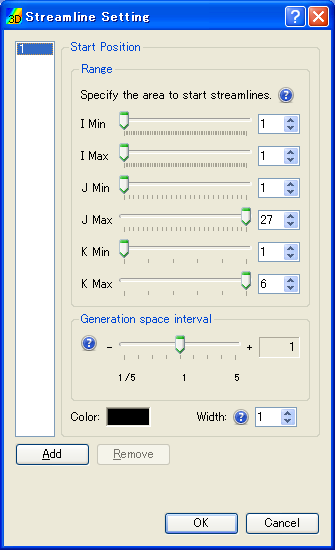
Figure 475 [Streamline Setting] dialog
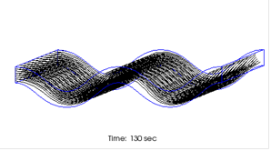
Figure 476 Example of the [Streamline] display
[Particles (auto)] (P)
Description: Setup the particle settings.
[Particles (auto)] is the function to generate particles in GUI, and simulate where where the particles will move to, using velocity in calculation result, and visualize the particles.
When you select [Particles], the [Particle Setting] dialog (Figure 477) will open. Set it and click on [OK]. Figure 478 shows an example of the [Particles] display.
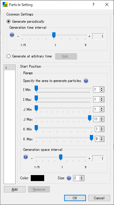
Figure 477 [Particle Setting] dialog
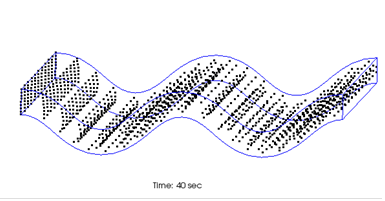
Figure 478 Example of the [Particles] display
[Particles] (R)
Description: Setup the particle settings.
[Particles] is the function to load particles output by solber, and visualize the particles.
When scalar attributes are output, user can change particle colors. When vector attributes are output, user can show arrows.
When you select [Property] menu in right-clicking menu of [Scalar] and [Vector] Folder under [Particles], the dialogs in Figure 479, Figure 480 will be shown. Please edit the setting, and click on [OK] button.
Figure 481 shows an example of the [Particles] display.
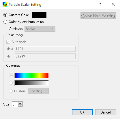
Figure 479 [Particle Scalar Setting] dialog
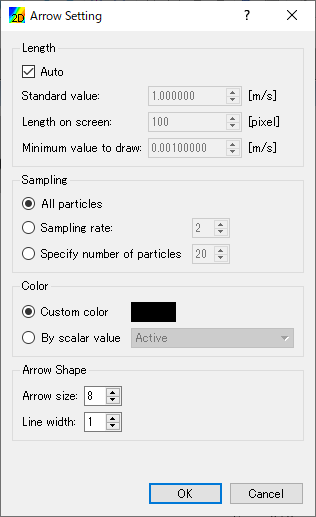
Figure 480 [Arrow Setting] dialog
Figure 481 Example of the [Particles] display
[Label]
Description: Show label based on calculation result values.
Label is the function to show label string defined using calculation results at grid nodes, cells, edges, etc.
Figure 482 shows an example of label.
Refer to Label display function for detail.
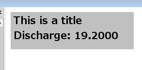
Figure 482 Example of [Label] display
[Title] (T)
Description: Setup the title settings.
When you select [Title], the [Title Setting] dialog (Figure 483) will open. Set it and click on [OK].
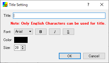
Figure 483 [Title Setting] dialog
[Time] (M)
Description: Setup the time settings.
When you select [Time], the [Time Setting] dialog (Figure 484) will open. Set it and click on [OK].
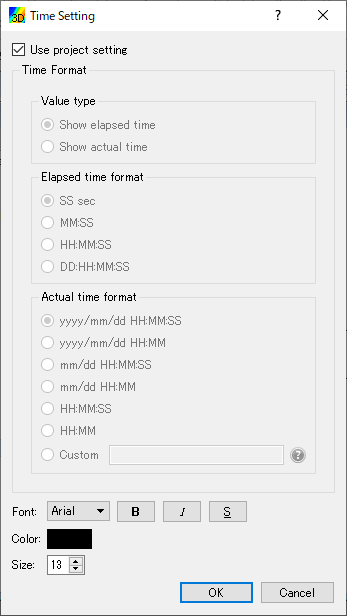
Figure 484 [Time Setting] dialog