[Graph Window]
The functions for opening a graph window that supports both “Time” and “Position” as X-axis, and easy to switch between them, are explained in this section.
[Open new Graph Window]
Either of the following actions opens a new graph window.
Menu bar: [Calculation Results] (R) –> [Open New Graph Window]
Operation Toolbar: ![]()
The [Data Source Setting] dialog (Figure 464) will open, so select the data to draw graph and click on [OK]. A new [Graph Window] window (Figure 466) will open that draws a graph for the data you selected.
When you select [Setting] on [Data Source Setting] dialog, the [Data Setting] dialog (Figure 465) is shown for the currently selected data, so modify the setting and click on [OK].
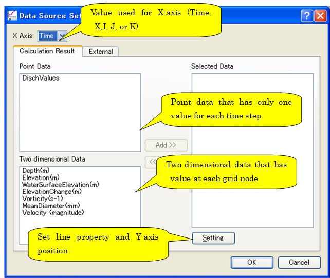
Figure 464 [Data Source Setting] dialog
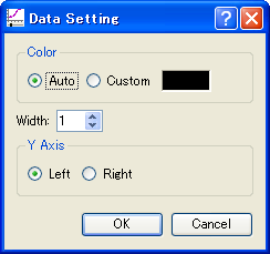
Figure 465 [Data Setting] dialog
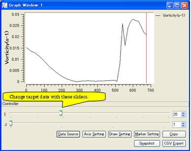
Figure 466 [Graph Window]
Note
Supporting calculation result defined at cell centers and cell edges
iRIC 3.0.11 and later supports drawing charts for calculation result defined at cell centers.
iRIC 3.0.18 and later supports drawing charts for calculation result defined at cell edges.
If calculation result defind at cell centers (or edges) exists, Combo box with label “Grid Location” is displayed, like in Figure 467, and you can draw charts for calculation result defined at cell centers or cell edges by selecting “CellCenter”, “EdgeI”, “EdgeJ”.
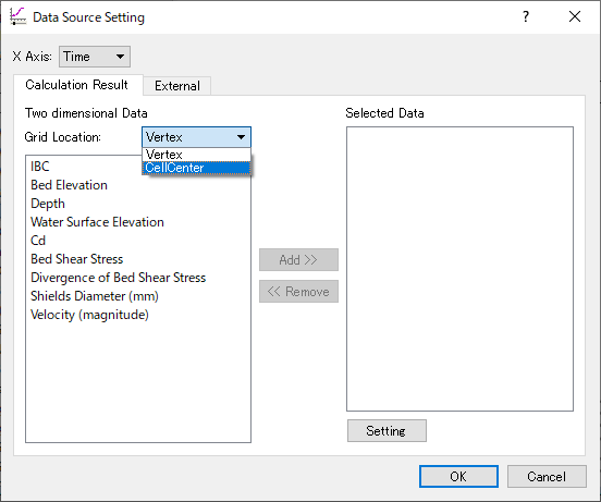
Figure 467 “Grid Location” selecting function
Note
Supporting drawing charts with calculation result interpolated to polylines
iRIC 3.0.14 and later supports drawing charts with calculation result interpolated to polylines.
Using this new feature, user can use chart windows to draw chart like followings:
Drawing chart for cross sections for solvers that uses unstructured grids
Drawing chart for arbitrary cross sections (not I or J lines of grids) for solvers that uses structured grids
To draw charts with calculation results interpolataed to polylines, on “Data source Setting” dialog, please select “Polyline” in “X Axis” combo box like in Figure 468, and in combo box “Polyline”, select the polyline on which you want to interpolate calculation result values and draw chart.
Please refer to Editing [Lines] for how to define polylines.
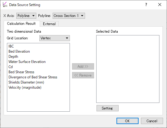
Figure 468 Example of setting up drawing charts for a polyline
[Data Source Setting] (D)
Description: Set data source setting.
When you select this, the [Data Source Setting] dialog (Figure 464) will open. Modify setting and click on [OK].
On the [Data Source Setting] dialog, you can import CSV files from [External] tab. Refer to Graph window external data file (*.csv) for the format of the CSV file to import.
[Axis Setting] (A)
Description: Set axis setting.
When you select this, the [Axis Setting] dialog (Figure 469) will open. Modify setting and click on [OK]. A new graph will be made according to the settings.
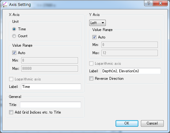
Figure 469 [Axis Setting] dialog
[Draw Setting] (D)
Description: Set the draw settings
When you select this, the [Draw Setting] dialog (Figure 470) will open. Modify setting and click on [OK]. A new graph will be made according to the settings.
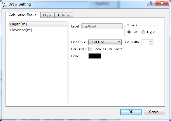
Figure 470 [Display Setting] dialog
[Marker Setting] (M)
Description: Set the marker settings
When you select this, the [Marker Setting] dialog (Figure 471) will open. Modify setting and click on [OK]. A new graph will be made according to the settings. Figure 472 shows an example of a [Graph Window] after setting up a marker.
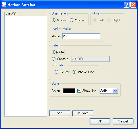
Figure 471 [Marker Setting] dialog
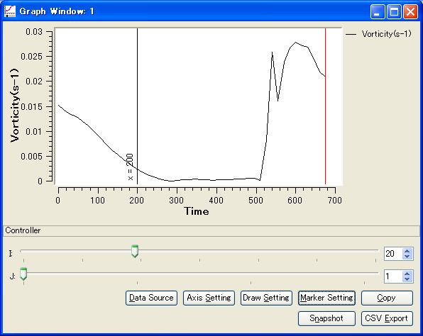
Figure 472 Example of the [Graph Window] after setting up a marker.
[Add KP Markers] (K)
Description: Add KP Markers for river survey data.
This function is available only when the following conditions are satisfied:
Graph for two-dimensional structured grid result is drawn.
X-axis is I-direction in the grid.
The grid is created using the algorithm “Create grid from river survey data”.
When you select this, the [Marker Setting] dialog (Figure 471) will open. Modify setting and click on [OK]. A new graph will be made according to the settings. Figure 473 shows an example of a [Graph Window] after setting up a marker.
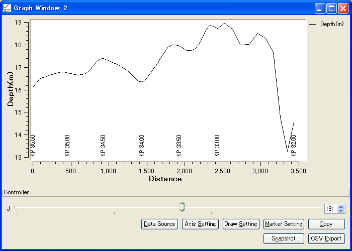
Figure 473 Example of the [Graph Window] after adding KP markers
[Copy] (C)
Description: Copy the calculation result. The copied data is fixed when the user changes time step or the setting on the controller.
Figure 474 shows an example of a [Graph Window] after copying data.
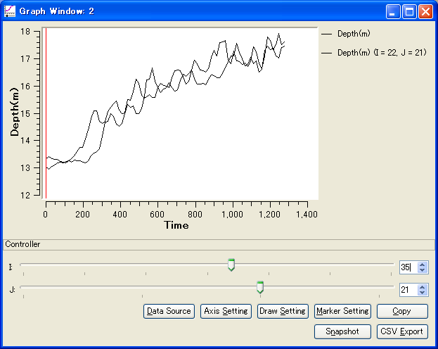
Figure 474 Example of the [Graph Window] after copying data
[Snapshot] (S)
Description: Save graph snapshots to image files.
When you select this, the [Snapshot Setting] dialog (Figure 475) will open. Setup setting, and click on [OK]. Saving snapshots will be started.

Figure 475 [Snapshot Setting] dialog
[CSV Export] (E)
Description: Save data to CSV files.
When you select this, the [CSV Export Setting] dialog (Figure 476) will open. Setup setting, and click on [OK]. Saving CSV files will be started.
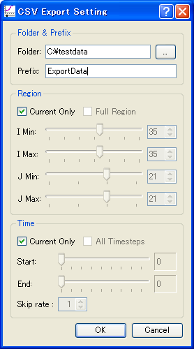
Figure 476 [CSV Export Setting] dialog